CFA Quantitative Methods

• Quantitative Methods are used to predict outcomes and measure results and are a core component of the CFA curriculum.
• CFA Quantitative Methods topic weight is 8-12% on the CFA Level I exam.
• At CFA Level I, candidates are expected to know the basics of Quantitative Methods. At CFA Level II, hypothesis testing builds on the knowledge of the previous level.
• UWorld offers study guides and tools to help you master CFA Quantitative Methods as you prepare for exam day.

CFA Quantitative Methods represents 14-21 of the 180 multiple-choice questions on the Level I CFA Exam. This means it deserves plenty of focus and attention as you prepare.As you dig into the reading material, highlight important sections, and re-read sections that need more clarity. Also, be sure to spend time on practice questions and mock exams to help you succeed on the exam and build a foundation for future CFA exams.

Understand the Concepts of Quantitative Methods, Don’t Just Memorize the Formulae

Memorization can be a helpful technique during your CFA preparation, but CFA Quantitative Methods require an understanding of the concepts rather than just rote memorization. In fact, understanding the logic of the concepts and how they relate to each other will help you stay focused and calm if you forget a formula.

Start Building Your Foundation With Quantitative Methods Early

Quantitative Methods expand beyond the specific questions you’ll face and the topic weights. That’s because they act as a foundational building block that crosses over into other areas of the CFA curriculum. So, developing a firm understanding of Quantitative Methods early will set you up for success at each CFA exam level.

Keep Practicing Quantitative Method Questions

As you build your knowledge of Quantitative Methods early, there are some specific approaches and tools that can help. One is through drilling questions, a process that will be especially useful as you prepare for the CFA Level I exam. And don’t forget to begin to familiarize yourself with your calculator during this stage as well.

Below is a table laying out the CFA Quantitative Methods Level I readings, subtopics, and a description for each. They’re all informed by the CFA Learning Outcome Statements (LOS) in order to find the most important concepts and formulas for each. This should serve as a regular reference as you prepare for the exam.

Reading 1 explores the time value of money. This reading asks candidates to interpret interest rates as required rates of return, discount rates, or opportunity costs. It also covers interest rates as the sum of real risk-free rates and premiums that compensate investors for taking on distinct types of risks.Additionally, candidates will be tasked with calculating and interpreting the effective annual rate, the future value (FV), and present value (PV) of a single sum of money, an ordinary annuity, an annuity due, perpetuity, and a series of unequal cash flows.

Finally, you’ll learn to solve time value of money problems for frequencies of compounding and demonstrate the use of a timeline in modeling and solving time value of money problems.

Present Value (PV) And Future Value (Fv) Of Cash Flows

Annuity Due vs Ordinary Annuity

• Ordinary annuity = cash flow at the end-of-time period.
• Annuity due = cash flow at the beginning-of-time period.

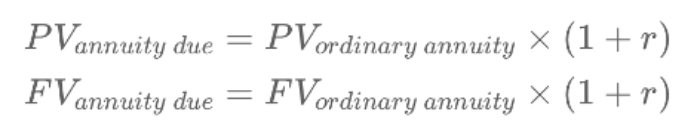
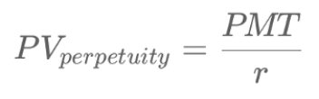
Perpetuity Is Just an Annuity With Infinite Life

Reading 2 covers Organizing, Visualizing, and Describing Data. The reading offers a foundation for understanding concepts that are a vital tool for investment professionals.Candidates will learn about core data types, organizing data into arrays and data tables, and summarizing data in frequency distributions and contingency tables.

Data visualization is introduced as well, using charts and graphs, followed by the key measures of central tendency. In addition, quantiles and their investment applications are covered, along with key measures of dispersion, the shape of data distributions, and a graphical introduction to covariance and the correlation between two variables.

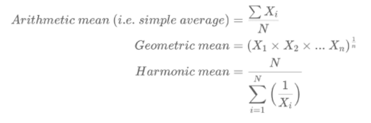
Arithmetic, Geometric, and Harmonic Mean

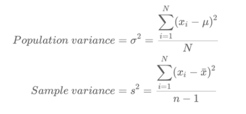
Population vs Sample Variance’s Formula

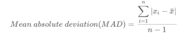
Mean Absolute Deviation (Mad)

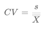
Coefficient of Variation (CV)

Reading 3 uses probabilities to predict outcomes when faced with uncertainty. Candidates will be offered essential tools needed to address real-world problems involving risk.

Issues, where these tools are helpful, include predicting investment manager performance, forecasting financial variables, and pricing bonds to compensate bondholders for default risk. You’ll also cover independence as it relates to the predictability of returns and financial variables, expectations from analysts looking ahead in their analysis and decisions, and variability, variance, or dispersion around expectation as a risk concept.

Conditional and Joint Probability

P(A | B) = P (AB) / P(B)
P(AB) = P(A | B) x P(B). But If A and B are independent, P(AB) = P(A) x P(B)
P(A or B) = P(A) + P(B)

Expected Value of a Random Variable X

E(X) = P(X1)X1 + P(X2)X2 + … + P(Xn)Xn

Probabilistic Variance

Correlation and Covariance of Returns

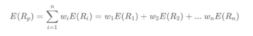
Expected Return on a Portfolio

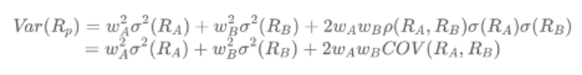
Variance of a 2 Stock Portfolio

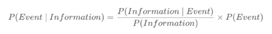
Bayes’ Formula

Reading 4 provides candidates with an overview of normal and non-normal distributions. Seven probability distributions and their investment uses are focused on. This includes the uniform, binomial, normal, lognormal, Student’s t-, chi-square, and F-distributions.Finally, there is an introduction to a computer-based tool that obtains information on complex investment problems called the Monte Carlo simulation.

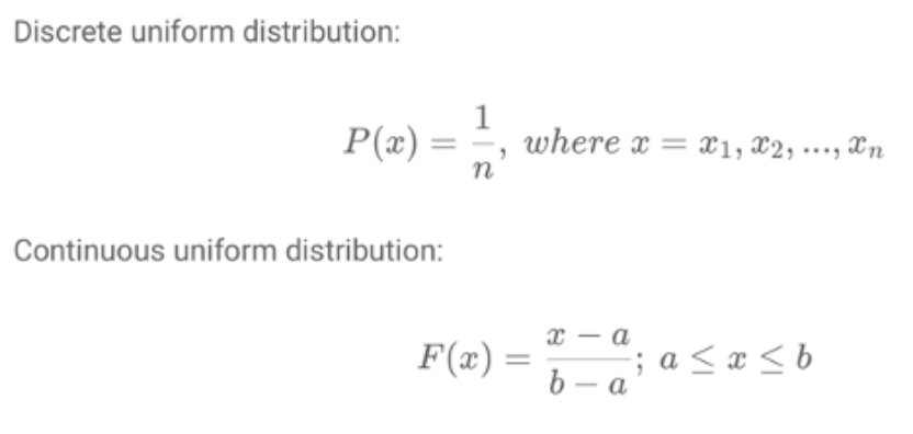
Uniform Distribution

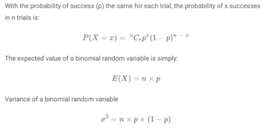
Binomial Distribution

Normal Distribution

The normal distribution is a continuous symmetric probability distribution that is completely described by two parameters: its mean, μ, and its variance σ2.

• 68% of observations lie in between μ +/- 1σ;
• 90% of observations lie in between μ +/- 1.65σ;
• 95% of observations lie in between μ +/- 1.96σ;
• 99% of observations lie in between μ +/- 2.58σ;

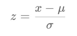
Compute Z-Score

Safety-First Ratio (SF Ratio)

Lognormal Distribution

The properties of lognormal distributions are:

• It cannot be negative.
• The upper end of its range extends to infinity.
• It is positively skewed.

Student’s T-Distribution

• T-distribution is defined by 1 parameter.
• It is symmetrical, with a similar bell-shaped distribution to Normal distribution, but has fatter tails and a lower peak.
• As df increases, t-distribution approximates Normal distribution.

Chi-Square Distribution

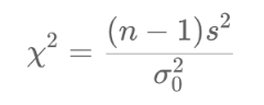
• A chi-square test is used to establish whether a hypothesized value of variance is equal to, less than, or greater than the true population variance.
• Chi-square distribution is the sum of squares of independent normal variables. Therefore, it cannot be negative.
• It is asymmetrical and is defined by one parameter.
• The shape of the curve is different for each df.
• As the df increase, the chi-square curve approximates the Normal distribution.

F-Distribution

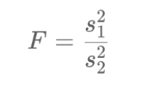
• F-distribution is a ratio of 2 chi-square distributions with 2 degrees of freedom, therefore it cannot be negative either.
• As both the numerator and the denominator’s degrees of freedoms increase, the f-distribution approximates the Normal distribution.

Monte Carlo Simulations

Monte Carlo simulations use computers to generate multiple random samples to produce a distribution of outcomes. It is used in financial planning, complex derivatives valuation, and VAR estimates.

Reading 5 uses samples to estimate the characteristics of a population. In investments, the mean is used as a measure of the central tendency of random variables. And when probability distribution of the random variable is unknown, they are made into probability statements about the population mean using the central limit theorem. The reading also dives into statistical estimation, central limit theorem and estimation, and the interpretation of statistical results based on financial data.

Central Limit Theorem

Central limit theorem states that when there are simple random samples each of size n from a population with a mean μ and variance σ2, the sample mean X approximately has a normal distribution with mean μ and variance σ2/n as n (sample size) becomes large.

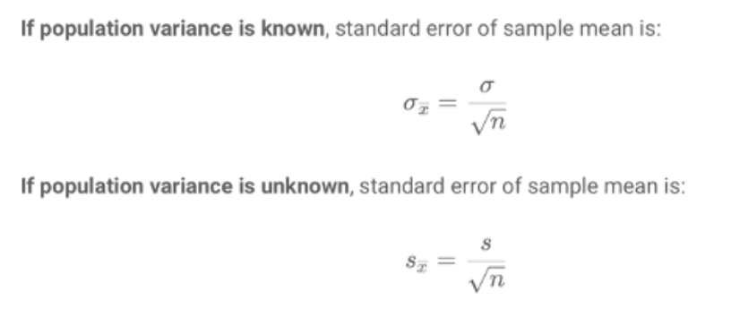
Standard Error

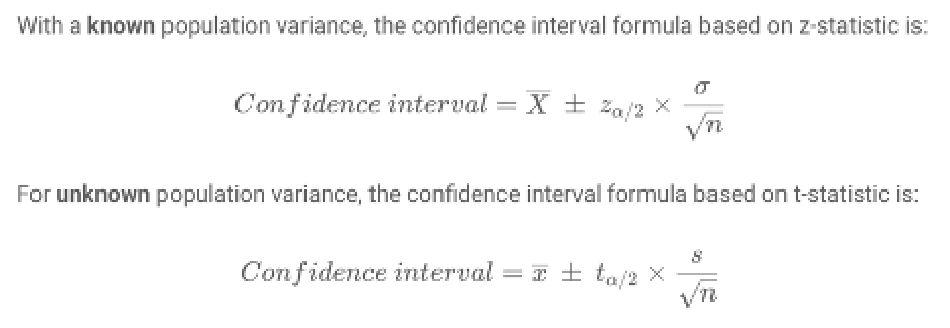
Confidence Intervals

Reading 6 helps you figure out the level of confidence you have in the conclusions you’ve found. This happens after a statistical test of a hypothesis, providing a clearer idea of the probability of the hypothesis. Along with hypothesis testing, the reading also offers tests having to do with mean, variance, and correlation.

Recapping the 6 Steps of Hypothesis Testing

1. State the hypothesis
2. Identify the appropriate test statistic
3. Specify the significance level
4. State the decision rule
5. Collect data and calculate the test statistic
6. Make a decision

Test Statistics: Population Mean

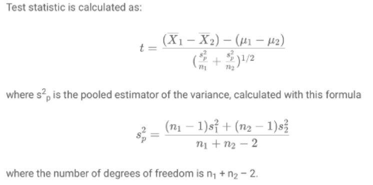
Tests Statistics: Differences Between Means (Independent Samples)

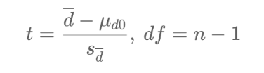
Test Statistics: Differences Between Means (Dependent Samples)

Tests Statistics: A Single Variance (Chi-Square Test)

Tests Statistics: Equality of Two Variances (F-Test)

Reading 7 introduces the simple linear regression model and its assumptions. This helps candidates learn the relationship between two variables and how to make predictions.

Basic Model of Simple Linear Regression

Assumptions of Simple Linear Regression

• Linear relationship between X and Y
• Homoscedasticity (constant variance of residuals for all observations)
• Independence between X and Y (residuals are uncorrelated for all observations)
• Normality of the residuals

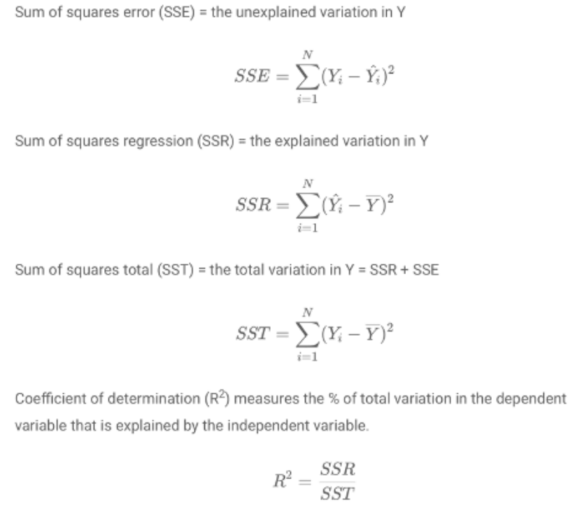
Analysis of Variance (Anova)